Probability and Statistics in Project Management

Project Estimation and PERT (Part 5): So far we have learned about the basics of PERT, how PERT is used to estimate activity completion time, and how the PERT formula was derived. We know that a project manager has to wear several hats. In this article, we are going to wear the probabilist and statistician hats and review the basic concepts of probability and statistics relevant to project estimation. It is certainly “out of scope” as far as the PMP exam is concerned. But if you ever wanted to learn the basics of random variables, distributions, mean, variance, standard deviation etc., without sacrificing a lot of precious time, then this article is just for you. I think it will give you the necessary foundation for understanding the concepts of project estimation and bring you one step closer to implementing theory into practice.

Random variable

The term random variable is a misnomer. Random variable is actually not a variable, but a function. The outcome of every event may not always be a number. For example, when you toss a coin, the outcome is a Head or a Tail. Random variable is a function which assigns a unique numerical value to every possible outcome of an event. For example, in a toss of a coin, how do we express these outcomes in a number? Let’s see.

Consider an experiment in which a coin is tossed three times. There are eight possible outcomes of this experiment:

HHH HHT HTH THH HTT THT TTH TTT

where H = Head and T = Tail

The number of Heads in these outcomes are:

3, 2, 2, 2, 1, 1, 1, 0

So, the number of times we can get a head in this experiment are 0, 1, 2 and 3.

In this experiment, we can say that the “Number of Heads” is a random variable. The numbers 0, 1, 2 and 3 are the “values” of the random variable.

If we express the random variable as X, then

X = Number of Heads in three tosses of a coin
Values of X = {0, 1, 2, 3}

As you can see, we have converted the outcomes from the toss of the coin experiment into numbers.

Types of Random Variables

Random variables are of 2 types:

• Continuous: A random variable with infinite number of values. Examples: The lifespan of people, and that of their LCD TVs and mobile phone batteries are examples of continuous random variables. They have an infinite number of possible values. Similarly, the number of miles a car will run before being scrapped, the length of a telephone conversation, the amount of rainfall in a season also fall in the same category. The duration of an activity on a project is also an example of a continuous random variable.
• Discrete: A random variable with countable number of distinct values. Examples: The score of students in an examination is a discrete random variable and so is the number of students who fail the exam. The experiment of three tosses of a coin (described above) is also an example of discrete random variable, with distinct values 0, 1, 2 and 3.
  

Distribution

If we plot a graph with the values of the random variable X on the x-axis and the probability of occurrence of the values on the y-axis, then the plot is known as a Distribution.

Probability Distribution Function (PDF)

The (mathematical) function that describes the shape of the Distribution is known as the Probability Distribution Function (PDF).

Common Probability Distributions

Some of the common distribution patterns are Uniform Distribution, Beta Distribution, Triangular Distribution and Normal Distribution.

Uniform Distribution

In the uniform distribution, each value of the random variable has equal probability of occurrence. For example, in a roll of a dice, each value (1 to 6) has an equal probability. The random variable is the score on each roll of the dice, and the values are 1 to 6. Each value has an equal probability of 1/6.

The uniform distribution can be continuous or discrete. The roll of a dice is an example of discrete uniform distribution. The uniform distribution looks like a rectangle, as shown in the following figure, where a is the minimum value and b is the maximum value of the distribution.

The uniform distribution is used in project management to determine rough estimates (range) when very little information is available about the project, and for risk management when several risks have equal probability of occurrence.

Triangular Distribution

The triangular distribution is a continuous probability distribution with a minimum value, a mode (most likely value), and a maximum value. The triangular distribution differs from the uniform distribution in that, the probability of the values of the random variable are not the same. The probability of the minimum, a and maximum value, b is zero, and the probability of the mode value, c is the highest for the entire distribution.

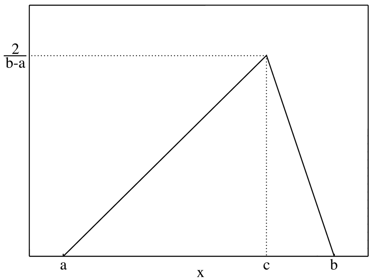
The triangular distribution is used in Project Management, often as an approximation to the beta distribution, to estimate activity duration. Assuming a triangular distribution, the expected activity duration (mean of the distribution) can be calculated using the simple average method.

Beta Distribution

The beta distribution is determined by 4 parameters:

• a - minimum value
• b - maximum value
• α - shape parameter
• β - shape parameter

Where a and b are finite numbers.

Natural events rarely have finite end points. However, Beta distribution approximates natural events quite well.

A form of beta distribution which looks like a rounded-off triangle is often used in project management to determine activity duration and cost. It models the optimistic (minimum), the pessimistic (maximum) and the most likely (mode) values quite well. The triangular distribution is considered a good approximation of the beta distribution.

Normal Distribution

A random variable which can take any value from -∞ to +∞, is said to follow a Normal Distribution. The normal distribution models natural events very well. In practice, the normal distribution is also used to model distributions with non-negative values. For example, the height of adults in a country is considered to follow a normal distribution, even though the height of a person can never be a negative number.

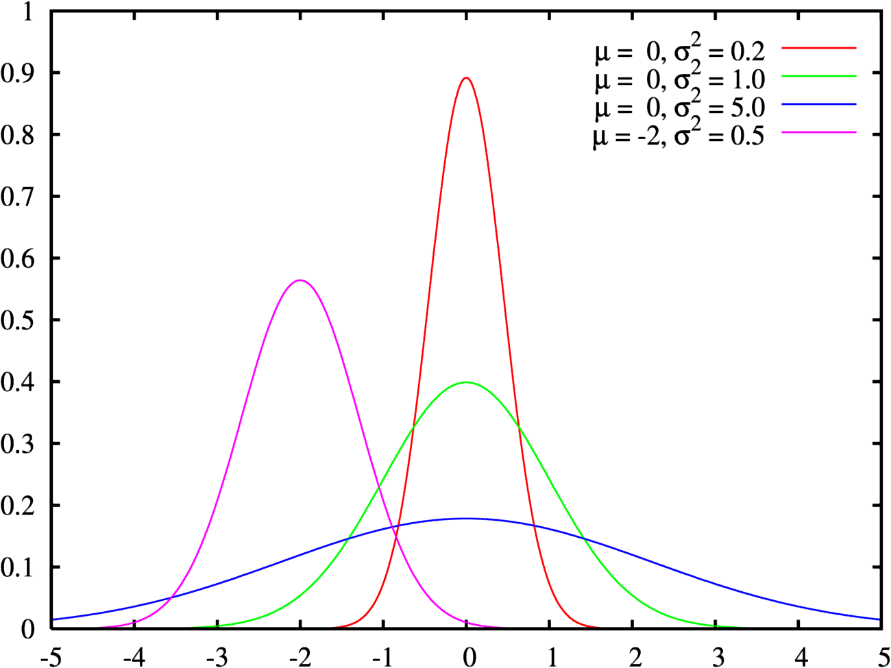
The normal distribution curve is symmetrical about the mean (expected value). The curve is also known as a bell-curve because of its resemblance to the shape of a bell. The simplest form of the normal distribution is known as the Standard Normal Distribution, which has a mean of 0 and variance of 1.

Because of it’s ability to accurately portray many real world events, the normal distribution has many practical applications. Be it height, weight or income of a population, or time and cost estimation in project management, all can be modeled fairly accurately using the normal distribution.

The normal distribution’s end points come very close to the horizontal axis but never actually touch it. This is unlike the beta distribution, whose end points touch the horizontal axis i.e. have a zero probability.

Expected Value or Mean (μ)

Expected value of a random variable is it’s mean or average value. This expected value is used in project management to represent the expected activity duration (or PERT estimate).

Variance (σ ^ 2)

Variance of a random variable is a measure of its spread. Variance is always non-negative. A small variance indicates that the values of the random variable are placed close to the mean, whereas a large variances indicates that the values are spread away from the mean.

Standard Deviation (σ)

Standard deviation is the square root of variance and is also always non-negative. It also gives a measure of the dispersion of values of a random variable.

Trivia: If both Variance and Standard Deviation give a measure of the spread of values of a random variable, then why do we need 2 variables to tell us the same thing?

The y-axis of the distribution curve gives the probability of occurrence of any value of a random variable. The ratio of the area under the curve between any two points a, b to the total area under the curve, gives the probability that the value of the random variable will lie between a and b. This is where standard deviation comes into play.

According to statistics, for the normal distribution, 68.2% values of a random variable fall within 1 standard deviation of the mean, 95.5% within 2 standard deviations of the mean and 99.7% within 3 standard deviations.

In other words, there’s a 68.2% probability that the value of a random variable will lie between the range [μ-σ, μ+σ], 95.5% probability to be within [μ-2σ, μ+2σ] and 99.7% probability to be within [μ-3σ, μ+3σ].

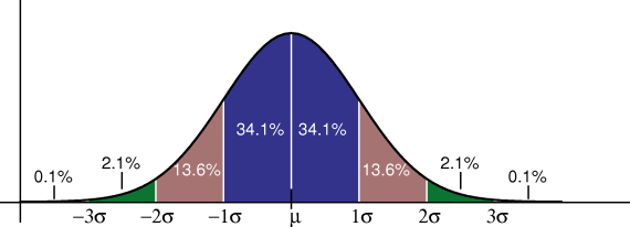
The area under the curve in the range [μ-σ, μ+σ] is 68.2% of the total area under the curve. This area is shown in blue. Similarly 95.5% area is covered in [μ-2σ, μ+2σ] range, and is the sum of the blue and brown colored regions. And lastly, 99.7% area is covered in [μ-3σ, μ+3σ] range and is the total area shown in blue, brown and green.

Central Limit Theorem

Central Limit Theorem (CLT) says that the mean of a large sample of independent random variables, each having a finite mean and variance, will be normally distributed. For CLT to be applicable, certain requirements should be met. The sample size should be fairly large (more than 30), the random variables should be independent of each other and should have the same type of distribution.

Let’s understand this with an example.

Say we have a set of coins with denominations of 1 to 999. The set of coins is the population and the denomination of each coin is a random variable. The mean of this entire population is 500. From this population, we select a sample of 50 coins, and take a mean of their denomination. It is possible that the mean of those 50 coins is less than 500, equal to 500, or even more than 500. Now if you repeatedly draw 50 coins from the set, calculate their mean, and plot the mean vs frequency graph, the resulting distribution will be close to normal. In general, the larger the sample size, the closer the resulting distribution will be to normal.

Let’s put this in project management perspective. We learned in the previous articles that the basic assumptions in PERT are that the individual activity durations are random variables and that they follow the beta distribution. Consider the individual activity durations as the random variables and the duration of activities on the critical path as the sample. In order to calculate the total project duration, we add up the PERT estimates of the activities on the critical path. According to CLT:

The total project duration is assumed to follow a normal distribution and the variance in project duration can be calculated by summing up the variances in the durations of activities on the critical path.

In real world project management, the conditions under which CLT is applicable, are not always met. For instance, the activities on a project, and hence their durations, are not always independent of each other. The critical path may not have 30 activities. We’ll discuss these issues in a follow-up article on the limitations of PERT.

With this we have come to the end of this post. As you know, this topic is a study in itself, and I cannot possibly cover it in enough detail. I’ve tried my best to summarize lot of information in a concise manner. Please use the comments section below to let me know whether you found it useful.

8-part series on Project Estimation and PERT

1. Get Intimate with PERT
2. Three Point Estimate - The Power of Three in Project Estimation
3. What is PERT?
4. The Magical PERT Formula
5. Probability and Statistics in Project Management (you are here)
6. PERT and CPM get Cozy
7. PMP Quiz Contest - Activity Duration Estimates
8. Standard Deviation and Project Duration Estimates

Image credit: Flickr / icma